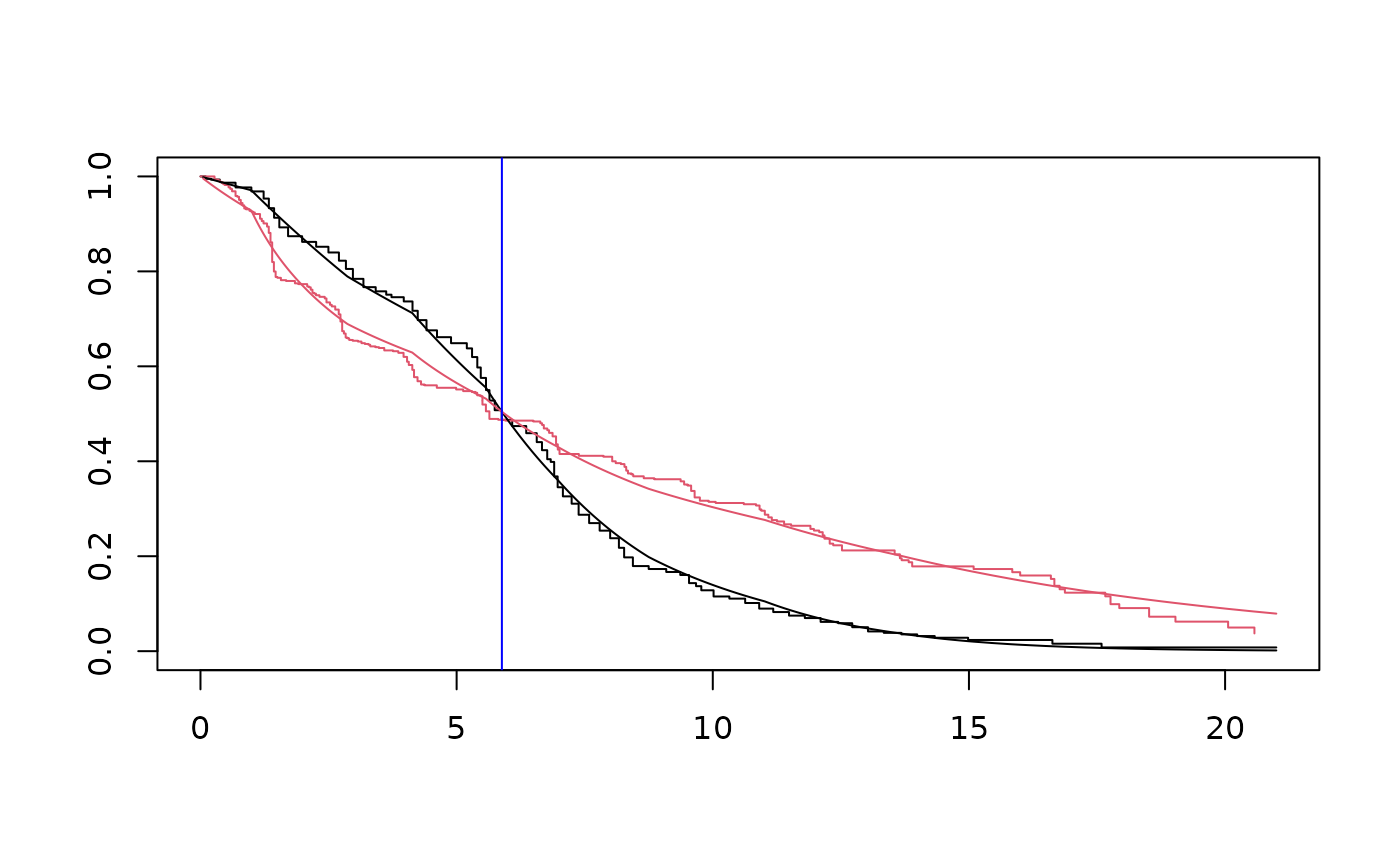
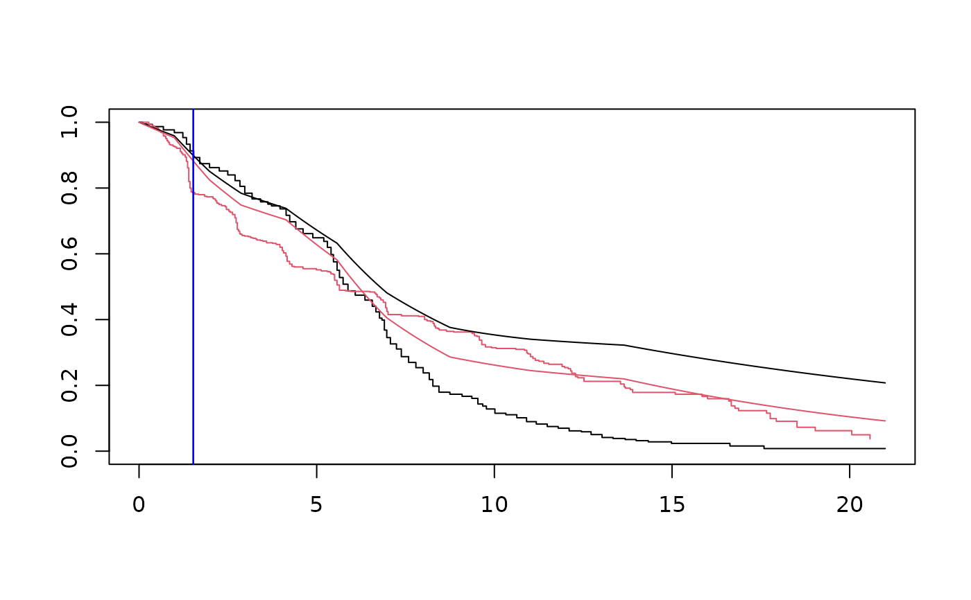
Computes the crossing survival times
Usage
# S3 method for yppe
crossTime(object, newdata1, newdata2, conf.level = 0.95, nboot = 1000, ...)
Arguments
- object
an object of class yppe
- newdata1
a data frame containing the first set of explanatory variables
- newdata2
a data frame containing the second set of explanatory variables
- conf.level
level of the confidence/credible intervals
- nboot
number of bootstrap samples (default nboot=1000); ignored if approach="bayes".
- ...
further arguments passed to or from other methods.
Examples
# \donttest{
# ML approach:
library(YPPE)
mle <- yppe(Surv(time, status)~arm, data=ipass, n_int=10, approach="mle", init = 0)
summary(mle)
#> Call:
#> yppe(formula = Surv(time, status) ~ arm, data = ipass, n_int = 10,
#>     approach = "mle", init = 0)
#>
#> Short-term coefficients:
#>     Estimate  StdErr z.value   p.value
#> arm  1.04152 0.16656  6.2533 4.019e-10 ***
#> ---
#> Signif. codes:  0 ‘***’ 0.001 ‘**’ 0.01 ‘*’ 0.05 ‘.’ 0.1 ‘ ’ 1
#>
#> Long-term coefficients:
#>     Estimate   StdErr z.value   p.value
#> arm -1.23838  0.08456 -14.645 < 2.2e-16 ***
#> ---
#> Signif. codes:  0 ‘***’ 0.001 ‘**’ 0.01 ‘*’ 0.05 ‘.’ 0.1 ‘ ’ 1
#>
#> ---
#> loglik = -2759.652   AIC = 5543.305
newdata1 <- data.frame(arm=0)
newdata2 <- data.frame(arm=1)
tcross <- crossTime(mle, newdata1, newdata2, nboot = 10)
tcross
#>       Est. 2.5% 97.5%
#> 1 5.883294   NA    NA
ekm <- survfit(Surv(time, status)~arm, data=ipass)
newdata <- data.frame(arm=0:1)
St <- survfit(mle, newdata)
plot(ekm, col=1:2)
with(St, lines(time, surv[[1]]))
with(St, lines(time, surv[[2]], col=2))
abline(v=tcross, col="blue")


# Bayesian approach:
bayes <- yppe(Surv(time, status)~arm, data=ipass, n_int=10, approach="bayes", chains=1, iter=10)
#>
#> SAMPLING FOR MODEL 'yppe' NOW (CHAIN 1).
#> Chain 1:
#> Chain 1: Gradient evaluation took 0.000804 seconds
#> Chain 1: 1000 transitions using 10 leapfrog steps per transition would take 8.04 seconds.
#> Chain 1: Adjust your expectations accordingly!
#> Chain 1:
#> Chain 1:
#> Chain 1: WARNING: No variance estimation is
#> Chain 1:          performed for num_warmup < 20
#> Chain 1:
#> Chain 1: Iteration: 1 / 10 [ 10%]  (Warmup)
#> Chain 1: Iteration: 2 / 10 [ 20%]  (Warmup)
#> Chain 1: Iteration: 3 / 10 [ 30%]  (Warmup)
#> Chain 1: Iteration: 4 / 10 [ 40%]  (Warmup)
#> Chain 1: Iteration: 5 / 10 [ 50%]  (Warmup)
#> Chain 1: Iteration: 6 / 10 [ 60%]  (Sampling)
#> Chain 1: Iteration: 7 / 10 [ 70%]  (Sampling)
#> Chain 1: Iteration: 8 / 10 [ 80%]  (Sampling)
#> Chain 1: Iteration: 9 / 10 [ 90%]  (Sampling)
#> Chain 1: Iteration: 10 / 10 [100%]  (Sampling)
#> Chain 1:
#> Chain 1:  Elapsed Time: 0.014 seconds (Warm-up)
#> Chain 1:                0.019 seconds (Sampling)
#> Chain 1:                0.033 seconds (Total)
#> Chain 1:
#> Warning: There were 1 chains where the estimated Bayesian Fraction of Missing Information was low. See
#> https://mc-stan.org/misc/warnings.html#bfmi-low
#> Warning: Examine the pairs() plot to diagnose sampling problems
#> Warning: The largest R-hat is 2.5, indicating chains have not mixed.
#> Running the chains for more iterations may help. See
#> https://mc-stan.org/misc/warnings.html#r-hat
summary(bayes)
#> Call:
#> yppe(formula = Surv(time, status) ~ arm, data = ipass, n_int = 10,
#>     approach = "bayes", chains = 1, iter = 10)
#>
#> Short-term coefficients:
#>      mean se_mean   sd   2.5%    25%    50%   75% 97.5% n_eff  Rhat
#> arm 0.125    0.15 0.28 -0.146 -0.035 -0.035 0.427 0.427 3.495 0.817
#>
#> Long-term coefficients:
#>      mean se_mean    sd   2.5%   25%   50%   75% 97.5% n_eff  Rhat
#> arm 0.886   0.523 0.978 -0.646 1.312 1.312 1.335 1.335 3.495 1.011
#>
#> ---
#> Inference for Stan model: yppe.
#> 1 chains, each with iter=10; warmup=5; thin=1;
#> post-warmup draws per chain=5, total post-warmup draws=5.
#>
newdata1 <- data.frame(arm=0)
newdata2 <- data.frame(arm=1)
tcross <- crossTime(bayes, newdata1, newdata2)
tcross
#>       Est.     2.5%    97.5%
#> 1 1.526788 1.526788 1.526788
ekm <- survfit(Surv(time, status)~arm, data=ipass)
newdata <- data.frame(arm=0:1)
St <- survfit(bayes, newdata)
plot(ekm, col=1:2)
with(St, lines(time, surv[[1]]))
with(St, lines(time, surv[[2]], col=2))
abline(v=tcross, col="blue")

# }
# }