To fit a survival model with the survstan package,
the user must choose among one of the available fitting functions
*reg(), where * stands for the type of regression model,
that is, aft for accelerated failure time (AFT) models,
ah for accelerates hazards (AH) models, ph for
proportional hazards (PO) models, po for proportional (PO)
models, yp for Yang & Prentice (YP) models, or
eh for extended hazard (EH) models.
The specification of the survival formula passed to the chosen
*reg() function follows the same syntax adopted in the
survival package, so that transition to the
survstan package can be smoothly as possible for those
familiar with the survival package.
The code below shows the model fitting of an AFT model with Weibull
baseline distribution using the survstan::aftreg()
function. For comparison purposes, we also fit to the same data the
Weibull regression model using survival::survreg()
function:
library(survstan)
library(dplyr)
library(GGally)

ovarian <- ovarian %>%
  mutate(
    across(c("rx", "resid.ds"), as.factor)
  )

survreg <- survreg(
  Surv(futime, fustat) ~ ecog.ps + rx,
  dist = "weibull", data = ovarian
)

aftreg <- aftreg(
  Surv(futime, fustat) ~ ecog.ps + rx,
  dist = "weibull", data = ovarian
)
Although the model specification is quite similar, there are some
important differences that the user should be aware of. While the model
fitted using the survival::survreg() function uses the log
scale representation of the AFT model with the presence of an intercept
term in the linear predictor, the survstan::aftreg()
considers the original time scale for model fitting without the presence
of the intercept term in the linear predictor.
To see that, let us summarize the fitted models:
summary(survreg)
#>
#> Call:
#> survreg(formula = Surv(futime, fustat) ~ ecog.ps + rx, data = ovarian,
#>     dist = "weibull")
#>              Value Std. Error     z       p
#> (Intercept)  7.425      0.929  7.99 1.3e-15
#> ecog.ps     -0.385      0.527 -0.73    0.47
#> rx2          0.529      0.529  1.00    0.32
#> Log(scale)  -0.123      0.252 -0.49    0.62
#>
#> Scale= 0.884
#>
#> Weibull distribution
#> Loglik(model)= -97.1   Loglik(intercept only)= -98
#>  Chisq= 1.74 on 2 degrees of freedom, p= 0.42
#> Number of Newton-Raphson Iterations: 5
#> n= 26
summary(aftreg)
#> Call:
#> aftreg(formula = Surv(futime, fustat) ~ ecog.ps + rx, data = ovarian,
#>     dist = "weibull")
#>
#> Accelerated failure time model fit with weibull baseline distribution:
#>
#> Regression coefficients:
#>         Estimate Std. Error z value Pr(>|z|)
#> ecog.ps  -0.3851     0.5270 -0.7307   0.4649
#> rx2       0.5287     0.5292  0.9991   0.3178
#>
#> Baseline parameters:
#>         Estimate Std. Error       2.5%      97.5%
#> alpha    1.13141    0.28535    0.69014     1.8548
#> gamma 1678.06655 1558.57309  271.78211 10360.9005
#> ---
#> loglik = -97.08449   AIC = 202.169

models <- list(survreg = survreg, aftreg = aftreg)
ggcoef_compare(models)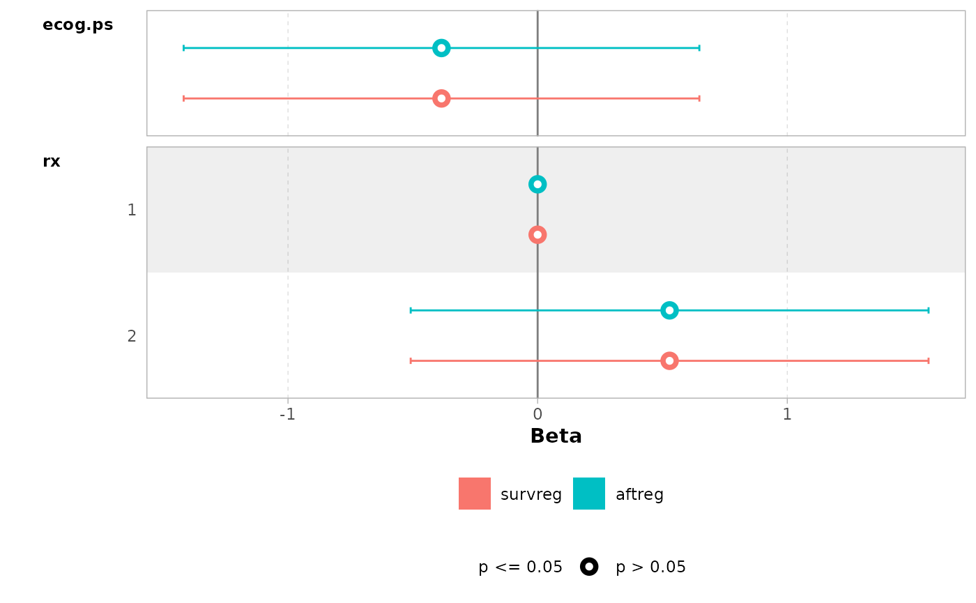
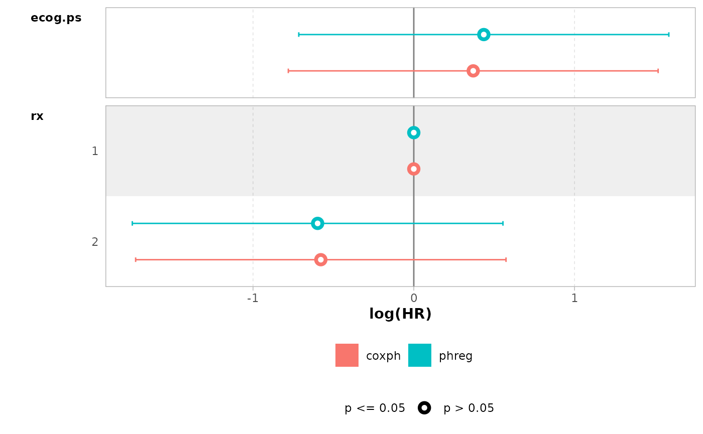
Next, we show how to fit a PH model using the
survstan::phreg() function. For comparison purposes, the
semiparametric Cox model is also fitted to the same data using the
function survival::coxph().
phreg <- phreg(
  Surv(futime, fustat) ~ ecog.ps + rx,
  data = ovarian, dist = "weibull"
)
coxph <- coxph(
  Surv(futime, fustat) ~ ecog.ps + rx, data = ovarian
)
coef(phreg)
#>    ecog.ps        rx2
#>  0.4355449 -0.5981575
coef(coxph)
#>    ecog.ps        rx2
#>  0.3697972 -0.5782271

models <- list(coxph = coxph, phreg = phreg)
ggcoef_compare(models)