Introduction
This vignette shows how to use the R package covid19br for downloading and exploring data from the COVID-19 pandemic in Brazil and the globe as well. The package downloads datasets from the following repositories:
The official Brazilian repository provided by the Brazilian government: https://covid.saude.gov.br;
The Johns Hopkins University’s repository: https://github.com/CSSEGISandData/COVID-19
The last repository has data on the COVID-19 pandemic at the global level (daily counts of confirmed cases, deaths, and recovered patients by countries and territories), and has been widely used all over the world as a reliable source of data information on the COVID-19 pandemic. The former repository, on the other hand, possesses data on the Brazilian territory by city, state, region, and national levels.
We hope that this package may be helpful to other researchers and scientists to understand and fight this terrible pandemic that has been plaguing the world.
Getting started with R package covid19br
We will get started by showing how to use the package to load into R data sets of the COVID-19 pandemic by downloading the COVID-19 data set from the official Brazilian repository https://covid.saude.gov.br
library(covid19br)
library(tidyverse)

# downloading the data (at national level):
brazil <- downloadCovid19("brazil")

# looking at the downloaded data:
glimpse(brazil)
#> Rows: 1,285
#> Columns: 9
#> $ date         <date> 2020-02-25, 2020-02-26, 2020-02-27, 2020-02-28, 2020-02-…
#> $ epi_week     <int> 9, 9, 9, 9, 9, 10, 10, 10, 10, 10, 10, 10, 11, 11, 11, 11…
#> $ newCases     <int> 0, 1, 0, 0, 1, 0, 0, 0, 1, 4, 6, 6, 6, 0, 9, 18, 25, 21, …
#> $ accumCases   <int> 0, 1, 1, 1, 2, 2, 2, 2, 3, 7, 13, 19, 25, 25, 34, 52, 77,…
#> $ newDeaths    <int> 0, 0, 0, 0, 0, 0, 0, 0, 0, 0, 0, 0, 0, 0, 0, 0, 0, 0, 0, …
#> $ accumDeaths  <int> 0, 0, 0, 0, 0, 0, 0, 0, 0, 0, 0, 0, 0, 0, 0, 0, 0, 0, 0, …
#> $ newRecovered <int> 0, 1, 1, 0, 1, 1, 0, 0, 1, 4, 6, 7, 6, 1, 6, 16, 23, 24, …
#> $ newFollowup  <int> 0, 0, 0, 1, 1, 1, 2, 2, 2, 3, 7, 12, 19, 24, 28, 36, 54, …
#> $ pop          <dbl> 210147125, 210147125, 210147125, 210147125, 210147125, 21…

# plotting the accumulative number of deaths:
ggplot(brazil, aes(x = date, y = accumDeaths)) +
  geom_point() +
  geom_path()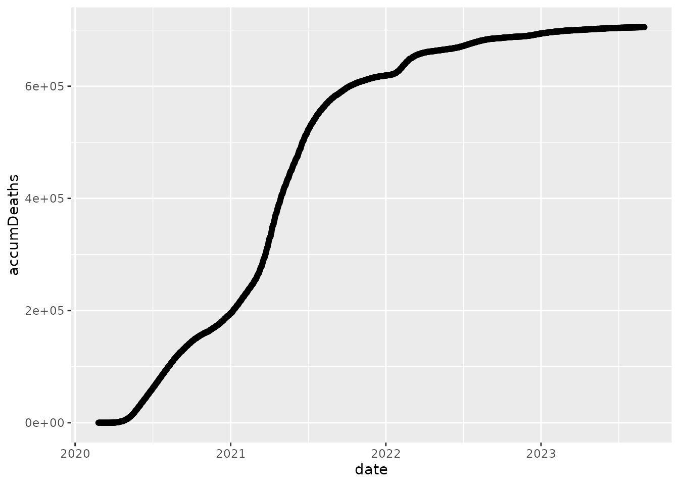
Next, will show how to draw a plot with the daily count of new deaths
along with its respective moving averarge. Here, we will use the
function pracma::movavg() to compute the moving
average.
library(pracma)

# computing the moving average:
brazil <- brazil %>%
  mutate(
    ma_newDeaths = movavg(newDeaths, n = 7, type = "s")
  )

# looking at the transformed data:
glimpse(brazil)
#> Rows: 1,285
#> Columns: 10
#> $ date         <date> 2020-02-25, 2020-02-26, 2020-02-27, 2020-02-28, 2020-02-…
#> $ epi_week     <int> 9, 9, 9, 9, 9, 10, 10, 10, 10, 10, 10, 10, 11, 11, 11, 11…
#> $ newCases     <int> 0, 1, 0, 0, 1, 0, 0, 0, 1, 4, 6, 6, 6, 0, 9, 18, 25, 21, …
#> $ accumCases   <int> 0, 1, 1, 1, 2, 2, 2, 2, 3, 7, 13, 19, 25, 25, 34, 52, 77,…
#> $ newDeaths    <int> 0, 0, 0, 0, 0, 0, 0, 0, 0, 0, 0, 0, 0, 0, 0, 0, 0, 0, 0, …
#> $ accumDeaths  <int> 0, 0, 0, 0, 0, 0, 0, 0, 0, 0, 0, 0, 0, 0, 0, 0, 0, 0, 0, …
#> $ newRecovered <int> 0, 1, 1, 0, 1, 1, 0, 0, 1, 4, 6, 7, 6, 1, 6, 16, 23, 24, …
#> $ newFollowup  <int> 0, 0, 0, 1, 1, 1, 2, 2, 2, 3, 7, 12, 19, 24, 28, 36, 54, …
#> $ pop          <dbl> 210147125, 210147125, 210147125, 210147125, 210147125, 21…
#> $ ma_newDeaths <dbl> 0.0000000, 0.0000000, 0.0000000, 0.0000000, 0.0000000, 0.…
After computing the desired moving average, it is convenient to reorganize the data to fit the so-called tidy data format. This task can be easily done with the aid of the function pivot_long():
deaths <- brazil %>%
  select(date, newDeaths, ma_newDeaths) %>%
  pivot_longer(
    cols = c("newDeaths", "ma_newDeaths"),
    values_to = "deaths", names_to = "type"
  ) %>%
  mutate(
    type = recode(type,
           ma_newDeaths = "moving average",
           newDeaths = "count",
    )
  )

# looking at the (tidy) data:
glimpse(deaths)
#> Rows: 2,570
#> Columns: 3
#> $ date   <date> 2020-02-25, 2020-02-25, 2020-02-26, 2020-02-26, 2020-02-27, 20…
#> $ type   <chr> "count", "moving average", "count", "moving average", "count", …
#> $ deaths <dbl> 0, 0, 0, 0, 0, 0, 0, 0, 0, 0, 0, 0, 0, 0, 0, 0, 0, 0, 0, 0, 0, …

# drawing the desired plot:
ggplot(deaths, aes(x = date, y=deaths, color = type)) +
  geom_point() +
  geom_path() +
  theme(legend.position="bottom")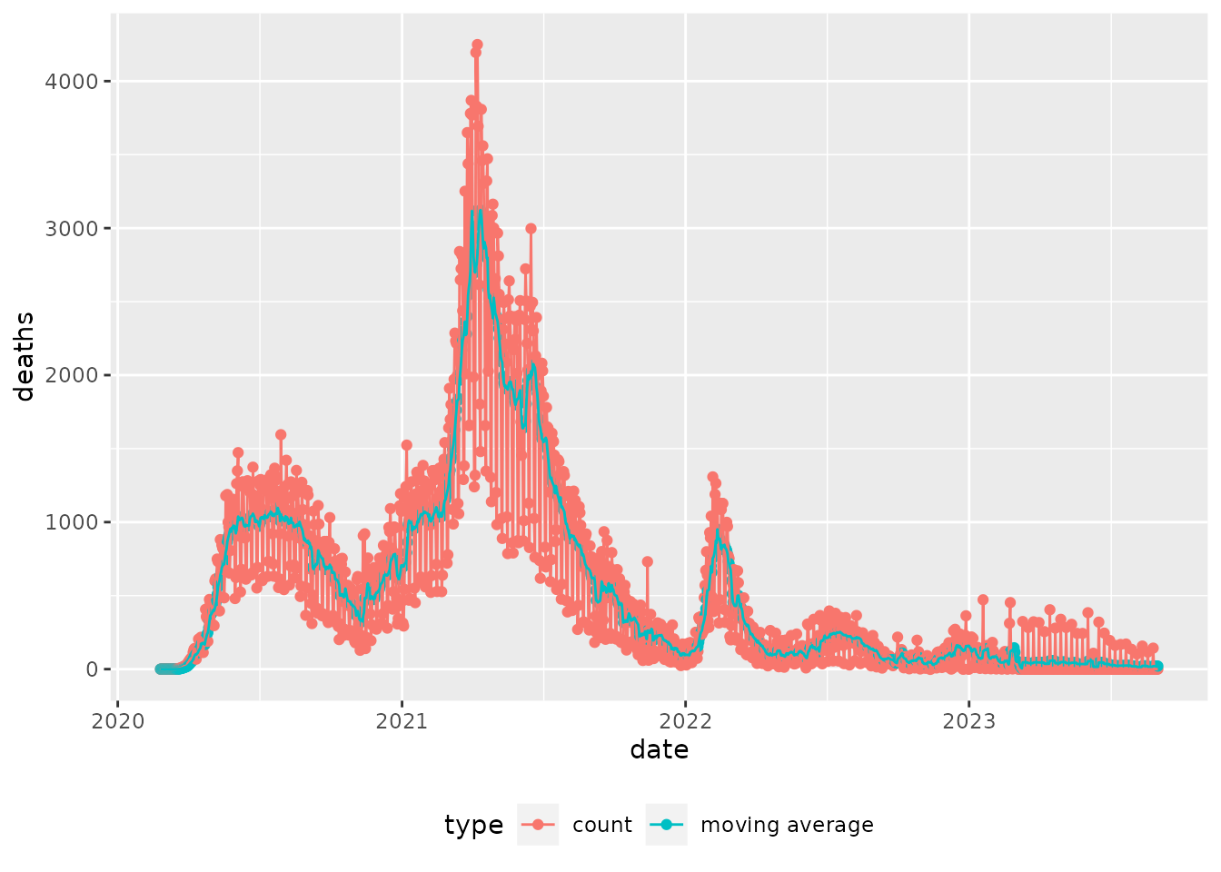
When dealing with epidemiological data we are often interested in
computing quantities such as incidence, mortality and lethality rates.
The function covid19br::add_epi_rates() can be used to add
those rates to the downloaded data, as shown below:
# downloading the data (region level):
regions <- downloadCovid19("regions")

# adding the rates to the downloaded data:
regions <- regions %>%
  add_epi_rates()

# looking at the data:
glimpse(regions)
#> Rows: 6,425
#> Columns: 13
#> $ region       <chr> "Midwest", "Midwest", "Midwest", "Midwest", "Midwest", "M…
#> $ date         <date> 2020-02-25, 2020-02-26, 2020-02-27, 2020-02-28, 2020-02-…
#> $ epi_week     <int> 9, 9, 9, 9, 9, 10, 10, 10, 10, 10, 10, 10, 11, 11, 11, 11…
#> $ newCases     <int> 0, 0, 0, 0, 0, 0, 0, 0, 0, 0, 0, 1, 0, 0, 0, 1, 0, 3, 4, …
#> $ accumCases   <int> 0, 0, 0, 0, 0, 0, 0, 0, 0, 0, 0, 1, 1, 1, 1, 2, 2, 5, 9, …
#> $ newDeaths    <int> 0, 0, 0, 0, 0, 0, 0, 0, 0, 0, 0, 0, 0, 0, 0, 0, 0, 0, 0, …
#> $ accumDeaths  <int> 0, 0, 0, 0, 0, 0, 0, 0, 0, 0, 0, 0, 0, 0, 0, 0, 0, 0, 0, …
#> $ newRecovered <int> NA, NA, NA, NA, NA, NA, NA, NA, NA, NA, NA, NA, NA, NA, N…
#> $ newFollowup  <int> NA, NA, NA, NA, NA, NA, NA, NA, NA, NA, NA, NA, NA, NA, N…
#> $ pop          <dbl> 16297074, 16297074, 16297074, 16297074, 16297074, 1629707…
#> $ incidence    <dbl> 0.000000000, 0.000000000, 0.000000000, 0.000000000, 0.000…
#> $ lethality    <dbl> 0, 0, 0, 0, 0, 0, 0, 0, 0, 0, 0, 0, 0, 0, 0, 0, 0, 0, 0, …
#> $ mortality    <dbl> 0, 0, 0, 0, 0, 0, 0, 0, 0, 0, 0, 0, 0, 0, 0, 0, 0, 0, 0, …
The function plotly::ggplotly() can be used to draw an
interactive plot as follows:
library(plotly)

p <- ggplot(regions, aes(x = date, y = mortality, color = region)) +
  geom_point() +
  geom_path()

ggplotly(p)
In our last example, we will obtain a table summarizing the for the 27 Brazilian capitals in 2023-09-01.
library(kableExtra)

cities <- downloadCovid19("cities")

capitals <- cities %>%
  filter(capital == TRUE, date == max(date)) %>%
  add_epi_rates() %>%
  select(region, state, city, newCases, newDeaths, accumCases, accumDeaths, incidence, mortality, lethality) %>%
  arrange(desc(lethality), desc(mortality), desc(incidence))

# printing the table:
capitals %>%
 kable(
    full_width = F,
    caption = "Summary of the COVID-19 pandemic in the 27 capitals of Brazilian states."
)| region | state | city | newCases | newDeaths | accumCases | accumDeaths | incidence | mortality | lethality |
|---|---|---|---|---|---|---|---|---|---|
| Southeast | SP | São Paulo | 0 | 0 | 1185972 | 45291 | 9679.806 | 369.6614 | 3.82 |
| Northeast | MA | São Luís | 0 | 0 | 78186 | 2763 | 7095.665 | 250.7523 | 3.53 |
| North | PA | Belém | 0 | 0 | 159248 | 5477 | 10668.132 | 366.9079 | 3.44 |
| North | AM | Manaus | 0 | 0 | 318613 | 9944 | 14596.775 | 455.5694 | 3.12 |
| Northeast | CE | Fortaleza | 0 | 0 | 409947 | 11817 | 15357.605 | 442.6934 | 2.88 |
| Southeast | RJ | Rio de Janeiro | 0 | 0 | 1341283 | 38306 | 19962.827 | 570.1228 | 2.86 |
| South | PR | Curitiba | 0 | 0 | 309818 | 8869 | 16026.962 | 458.7956 | 2.86 |
| Northeast | BA | Salvador | 0 | 0 | 339762 | 9160 | 11828.724 | 318.9030 | 2.70 |
| Midwest | MT | Cuiabá | 0 | 0 | 154410 | 3749 | 25207.862 | 612.0347 | 2.43 |
| Northeast | AL | Maceió | 0 | 0 | 133505 | 3231 | 13102.239 | 317.0917 | 2.42 |
| Northeast | PE | Recife | 0 | 0 | 308252 | 6829 | 18730.446 | 414.9534 | 2.22 |
| Midwest | MS | Campo Grande | 0 | 0 | 217183 | 4714 | 24239.661 | 526.1266 | 2.17 |
| North | RO | Porto Velho | 0 | 0 | 130194 | 2761 | 24586.059 | 521.3920 | 2.12 |
| Northeast | PI | Teresina | 0 | 0 | 144550 | 3030 | 16713.978 | 350.3518 | 2.10 |
| Northeast | RN | Natal | 0 | 0 | 157079 | 3225 | 17766.666 | 364.7687 | 2.05 |
| South | RS | Porto Alegre | 0 | 0 | 337156 | 6719 | 22722.913 | 452.8327 | 1.99 |
| Northeast | PB | João Pessoa | 0 | 0 | 179645 | 3302 | 22205.398 | 408.1507 | 1.84 |
| Southeast | MG | Belo Horizonte | 0 | 0 | 472778 | 8451 | 18820.256 | 336.4158 | 1.79 |
| Midwest | GO | Goiânia | 0 | 0 | 471089 | 8095 | 31072.156 | 533.9312 | 1.72 |
| North | AP | Macapá | 0 | 0 | 99730 | 1616 | 19814.157 | 321.0636 | 1.62 |
| Northeast | SE | Aracaju | 0 | 0 | 172080 | 2629 | 26191.263 | 400.1443 | 1.53 |
| North | AC | Rio Branco | 0 | 0 | 88007 | 1226 | 21606.407 | 300.9926 | 1.39 |
| Midwest | DF | Brasília | 0 | 0 | 912165 | 11886 | 30251.540 | 394.1938 | 1.30 |
| North | RR | Boa Vista | 0 | 0 | 141081 | 1654 | 35339.781 | 414.3152 | 1.17 |
| Southeast | ES | Vitória | 0 | 0 | 151337 | 1463 | 41794.602 | 404.0354 | 0.97 |
| North | TO | Palmas | 0 | 0 | 90929 | 735 | 30398.125 | 245.7150 | 0.81 |
| South | SC | Florianópolis | 0 | 0 | 172829 | 1357 | 34498.666 | 270.8729 | 0.79 |