When dealing with epidemiological data, we are often interested in visualizing the data through different types of maps. Drawing maps in R nowadays is a simple task provided the necessary geometry is available along with the data.
The function covid19br::add_geo() can be used to add the
geometry to the downloaded data as follows:
library(covid19br)
library(tidyverse)
# downloading data at state level:
cities <- downloadCovid19("cities")
# adding the geometry to the data:
cities_geo <- cities %>%
filter(date == max(date)) %>%
add_geo()
# looking at the data:
glimpse(cities_geo)
#> Rows: 5,570
#> Columns: 28
#> $ region <chr> "North", "North", "North", "North", "North", "North"…
#> $ state <chr> "RO", "RO", "RO", "RO", "RO", "RO", "RO", "RO", "RO"…
#> $ city <chr> "Alta Floresta D'Oeste", "Ariquemes", "Cabixi", "Cac…
#> $ state_code <dbl> 11, 11, 11, 11, 11, 11, 11, 11, 11, 11, 11, 11, 11, …
#> $ city_code <dbl> 110001, 110002, 110003, 110004, 110005, 110006, 1100…
#> $ healthRegion_code <int> 11005, 11001, 11006, 11002, 11006, 11006, 11006, 110…
#> $ healthRegion <chr> "ZONA DA MATA", "VALE DO JAMARI", "CONE SUL", "CAFE"…
#> $ date <date> 2023-04-26, 2023-04-26, 2023-04-26, 2023-04-26, 202…
#> $ epi_week <int> 17, 17, 17, 17, 17, 17, 17, 17, 17, 17, 17, 17, 17, …
#> $ pop <dbl> 22945, 107863, 5312, 85359, 16323, 15882, 7391, 1833…
#> $ accumCases <int> 9182, 36928, 1919, 31696, 6592, 4835, 2338, 4799, 79…
#> $ newCases <int> 0, 0, 0, 0, 0, 0, 0, 0, 0, 0, 0, 0, 0, 0, 0, 0, 0, 0…
#> $ accumDeaths <int> 84, 565, 23, 357, 74, 56, 25, 45, 92, 246, 209, 670,…
#> $ newDeaths <int> 0, 0, 0, 0, 0, 0, 0, 0, 0, 0, 0, 0, 0, 0, 0, 0, 0, 0…
#> $ newRecovered <int> NA, NA, NA, NA, NA, NA, NA, NA, NA, NA, NA, NA, NA, …
#> $ newFollowup <int> NA, NA, NA, NA, NA, NA, NA, NA, NA, NA, NA, NA, NA, …
#> $ metrop_area <int> 0, 0, 0, 0, 0, 0, 0, 0, 0, 0, 0, 0, 0, 0, 0, 0, 1, 0…
#> $ capital <lgl> FALSE, FALSE, FALSE, FALSE, FALSE, FALSE, FALSE, FAL…
#> $ DHI <dbl> 0.641, 0.702, 0.650, 0.718, 0.692, 0.685, 0.613, 0.6…
#> $ EDHI <dbl> 0.526, 0.600, 0.559, 0.620, 0.602, 0.584, 0.473, 0.4…
#> $ LDHI <dbl> 0.763, 0.806, 0.757, 0.821, 0.799, 0.814, 0.774, 0.7…
#> $ IDHI <dbl> 0.657, 0.716, 0.650, 0.727, 0.688, 0.676, 0.630, 0.6…
#> $ region_code <dbl> 1, 1, 1, 1, 1, 1, 1, 1, 1, 1, 1, 1, 1, 1, 1, 1, 1, 1…
#> $ mesoregion_code <int> 1102, 1102, 1102, 1102, 1102, 1102, 1102, 1101, 1102…
#> $ microregion_code <int> 11006, 11003, 11008, 11006, 11008, 11008, 11008, 110…
#> $ area [km^2] 7112.842 [km^2], 4439.795 [km^2], 1319.708 [km^2], …
#> $ demoDens [1/km^2] 3.225855 [1/km^2], 24.294590 [1/km^2], 4.025134 […
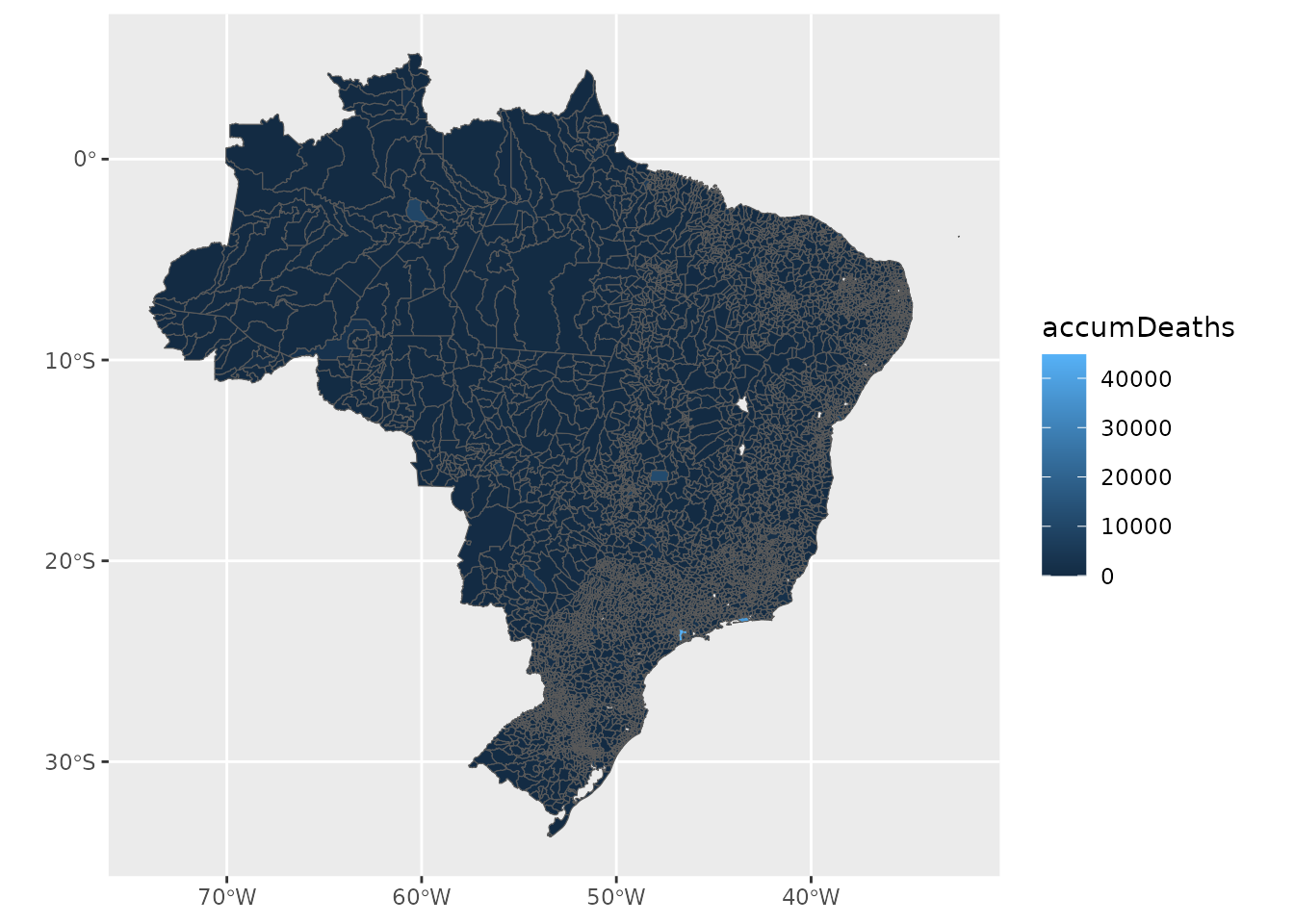
#> $ geometry <MULTIPOLYGON [°]> MULTIPOLYGON (((-62.05044 -..., MULTIPO…The map of the accumulated number of deaths by city can be easily drawn using the package ggplot2 as illustrated below:
Suppose now that we want to draw a map with the incidence of the COVID-19 in the cities belonging to Minas Gerais (MG) state. This can be done as follows:
mg <- cities_geo %>%
  filter(state == "MG") %>%
  add_epi_rates()

ggplot(mg) +
geom_sf(aes(fill = incidence)) 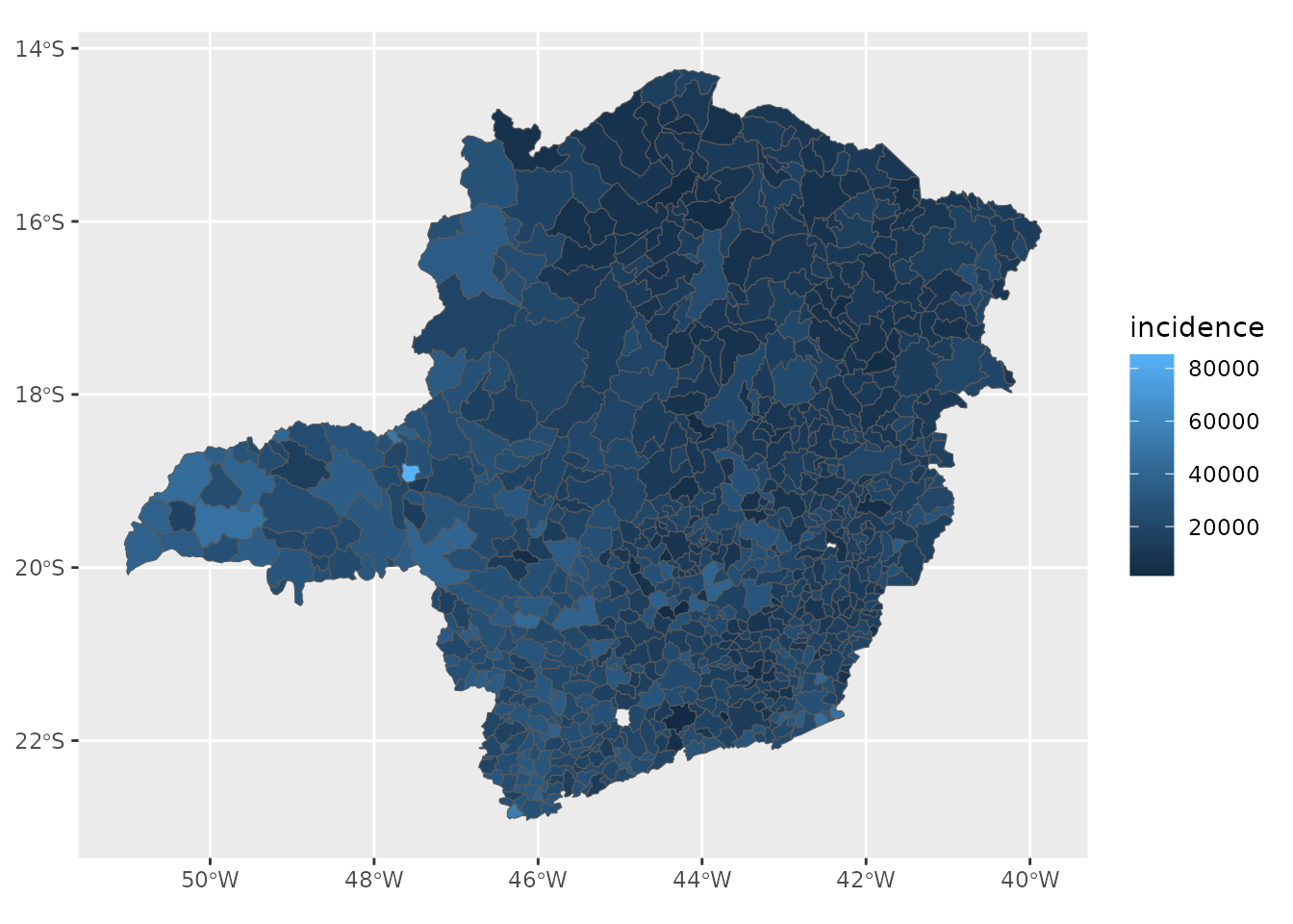
Next, we will show how to draw interactive maps using the package leaflet. As an illustration, we will consider the lethality by states:
library(leaflet)

# downloading data at state level:
states <- downloadCovid19("states")

# adding the geometry to the data:
states_geo <- states %>%
  filter(date == max(date)) %>%
  add_geo() %>%
  add_epi_rates()

# looking at the data:
glimpse(states_geo)
#> Rows: 27
#> Columns: 23
#> $ region       <chr> "North", "North", "North", "North", "North", "North", "No…
#> $ state        <chr> "RO", "AC", "AM", "RR", "PA", "AP", "TO", "MA", "PI", "CE…
#> $ date         <date> 2023-04-26, 2023-04-26, 2023-04-26, 2023-04-26, 2023-04-…
#> $ epi_week     <int> 17, 17, 17, 17, 17, 17, 17, 17, 17, 17, 17, 17, 17, 17, 1…
#> $ newCases     <int> 0, 0, 0, 0, 0, 0, 0, 0, 0, 0, 0, 0, 0, 0, 0, 0, 0, 0, 0, …
#> $ accumCases   <int> 484458, 162454, 636254, 183901, 878153, 185984, 367704, 4…
#> $ newDeaths    <int> 0, 0, 0, 0, 0, 0, 0, 0, 0, 0, 0, 0, 0, 0, 0, 0, 0, 0, 0, …
#> $ accumDeaths  <int> 7435, 2047, 14473, 2193, 19079, 2169, 4238, 11065, 8369, …
#> $ newRecovered <int> NA, NA, NA, NA, NA, NA, NA, NA, NA, NA, NA, NA, NA, NA, N…
#> $ newFollowup  <int> NA, NA, NA, NA, NA, NA, NA, NA, NA, NA, NA, NA, NA, NA, N…
#> $ pop          <dbl> 1777225, 881935, 4144597, 605761, 8602865, 845731, 157286…
#> $ state_code   <dbl> 11, 12, 13, 14, 15, 16, 17, 21, 22, 23, 24, 25, 26, 27, 2…
#> $ DHI          <dbl> 33.490, 12.894, 35.037, 9.153, NA, 10.285, 88.950, 125.03…
#> $ EDHI         <dbl> 26.854, 9.949, 27.090, 7.488, NA, 8.799, 75.863, 106.031,…
#> $ LDHI         <dbl> 41.019, 16.865, 47.464, 11.971, NA, 12.543, 109.778, 160.…
#> $ IDHI         <dbl> 34.225, 12.880, 33.797, 8.668, NA, 9.902, 84.859, 115.371…
#> $ region_code  <dbl> 1, 1, 1, 1, 1, 1, 1, 2, 2, 2, 2, 2, 2, 2, 2, 2, 3, 3, 3, …
#> $ area         [km^2] 238719.84 [km^2], 164806.00 [km^2], 1565986.97 [km^2], 2…
#> $ demoDens     [1/km^2] 7.444815 [1/km^2], 5.351353 [1/km^2], 2.646636 [1/km^2…
#> $ geometry     <GEOMETRY [°]> POLYGON ((-60.70931 -13.693..., POLYGON ((-68.38…
#> $ incidence    <dbl> 27259.238, 18420.178, 15351.408, 30358.673, 10207.681, 21…
#> $ lethality    <dbl> 1.53, 1.26, 2.27, 1.19, 2.17, 1.17, 1.15, 2.24, 1.95, 1.9…
#> $ mortality    <dbl> 418.3488, 232.1033, 349.2016, 362.0240, 221.7750, 256.464…

reds = colorBin("Reds", domain = states_geo$lethality, bins = 5)
mymap <- states_geo %>%
  leaflet() %>%
  addPolygons(fillOpacity = 1,
              weight = 1,
              smoothFactor = 0.2,
              color = "gray",
              fillColor = ~ reds(lethality),
              popup = paste0(states_geo$state, ":  ",  states_geo$lethality, 2)
  ) %>%
  addLegend(position = "bottomright",
            pal = reds, values = ~states_geo$lethality,
            title = "lethality")
mymap
Depending on the computer in use, the R session might crash if the geometry is added to the whole downloaded dataset (this is particularly true for the dataset at the city level) due to the lack of RAM. Therefore, we advise the users to filter the data by a desirable date before the addition of the geometry.
For the next example we will draw a bubble map with the 27 capitals of Brazilian states.
library(sf)
#> Linking to GEOS 3.10.2, GDAL 3.4.1, PROJ 8.2.1; sf_use_s2() is TRUE
library(ggrepel)

# getting the data:

states_geo <- downloadCovid19("states") %>%
  filter(date == max(date)) %>%
  add_geo()
#> Downloading COVID-19 data from the official Brazilian repository: https://covid.saude.gov.br/
#> Please, be patient...
#> Done!
#> Joining with `by = join_by(region, state, pop, state_code)`

capitals <- downloadCovid19("cities") %>%
  filter(date == max(date), capital == TRUE) %>%
  add_geo() %>%
  add_epi_rates()
#> Downloading COVID-19 data from the official Brazilian repository: https://covid.saude.gov.br/
#> Please, be patient...
#> Done!
#> Joining with `by = join_by(region, state, city, state_code, city_code, pop)`

# adding the coordinates associated with each capital:
capitals <- cbind(capitals, st_coordinates(st_centroid(capitals)))
#> Warning: st_centroid assumes attributes are constant over geometries
# looking at the data:
glimpse(capitals)
#> Rows: 27
#> Columns: 33
#> $ region            <chr> "North", "North", "North", "North", "North", "North"…
#> $ state             <chr> "RO", "AC", "AM", "RR", "PA", "AP", "TO", "MA", "PI"…
#> $ city              <chr> "Porto Velho", "Rio Branco", "Manaus", "Boa Vista", …
#> $ state_code        <dbl> 11, 12, 13, 14, 15, 16, 17, 21, 22, 23, 24, 25, 26, …
#> $ city_code         <dbl> 110020, 120040, 130260, 140010, 150140, 160030, 1721…
#> $ healthRegion_code <int> 11004, 12002, 13001, 14001, 15006, 16001, 17006, 210…
#> $ healthRegion      <chr> "MADEIRA-MAMORE", "BAIXO ACRE E PURUS", "MANAUS, ENT…
#> $ date              <date> 2023-04-26, 2023-04-26, 2023-04-26, 2023-04-26, 202…
#> $ epi_week          <int> 17, 17, 17, 17, 17, 17, 17, 17, 17, 17, 17, 17, 17, …
#> $ pop               <dbl> 529544, 407319, 2182763, 399213, 1492745, 503327, 29…
#> $ accumCases        <int> 129376, 86972, 318040, 139775, 158424, 99612, 89942,…
#> $ newCases          <int> 0, 0, 0, 0, 0, 0, 0, 0, 0, 0, 0, 0, 0, 0, 0, 0, 0, 0…
#> $ accumDeaths       <int> 2748, 1211, 9940, 1650, 5448, 1616, 734, 2758, 3015,…
#> $ newDeaths         <int> 0, 0, 0, 0, 0, 0, 0, 0, 0, 0, 0, 0, 0, 0, 0, 0, 0, 0…
#> $ newRecovered      <int> NA, NA, NA, NA, NA, NA, NA, NA, NA, NA, NA, NA, NA, …
#> $ newFollowup       <int> NA, NA, NA, NA, NA, NA, NA, NA, NA, NA, NA, NA, NA, …
#> $ metrop_area       <int> 1, 1, 1, 1, 1, 1, 1, 1, 1, 1, 1, 1, 1, 1, 1, 1, 1, 1…
#> $ capital           <lgl> TRUE, TRUE, TRUE, TRUE, TRUE, TRUE, TRUE, TRUE, TRUE…
#> $ DHI               <dbl> 0.736, 0.727, 0.737, 0.752, 0.746, 0.733, 0.788, 0.7…
#> $ EDHI              <dbl> 0.638, 0.661, 0.658, 0.708, 0.673, 0.663, 0.749, 0.7…
#> $ LDHI              <dbl> 0.819, 0.798, 0.826, 0.816, 0.822, 0.820, 0.827, 0.8…
#> $ IDHI              <dbl> 0.764, 0.729, 0.738, 0.737, 0.751, 0.723, 0.789, 0.7…
#> $ region_code       <dbl> 1, 1, 1, 1, 1, 1, 1, 2, 2, 2, 2, 2, 2, 2, 2, 2, 3, 3…
#> $ mesoregion_code   <int> 1101, 1202, 1303, 1401, 1503, 1602, 1702, 2101, 2202…
#> $ microregion_code  <int> 11001, 12004, 13007, 14001, 15007, 16003, 17006, 210…
#> $ area              [km^2] 34246.51028 [km^2], 8878.62792 [km^2], 11443.62930 …
#> $ demoDens          [1/km^2] 15.46271 [1/km^2], 45.87635 [1/km^2], 190.74045 […
#> $ incidence         <dbl> 24431.586, 21352.306, 14570.524, 35012.637, 10612.93…
#> $ lethality         <dbl> 2.12, 1.39, 3.13, 1.18, 3.44, 1.62, 0.82, 3.58, 2.14…
#> $ mortality         <dbl> 518.9370, 297.3100, 455.3861, 413.3132, 364.9652, 32…
#> $ X                 <dbl> -64.30327, -68.37132, -60.26007, -60.71681, -48.4596…
#> $ Y                 <dbl> -9.1538509, -10.0656694, -2.6255126, 3.1191952, -1.2…
#> $ geometry          <MULTIPOLYGON [°]> MULTIPOLYGON (((-62.26889 -..., MULTIPO…

# drawing some maps:
incidence <- ggplot() +
  geom_sf(data = states_geo, aes(geometry=geometry)) +
  geom_point(data = capitals, aes(x=X, y=Y, size=incidence, alpha=incidence), color = "orange") +
  geom_text_repel( data=capitals, aes(x=X, y=Y, label=city), size=3)
incidence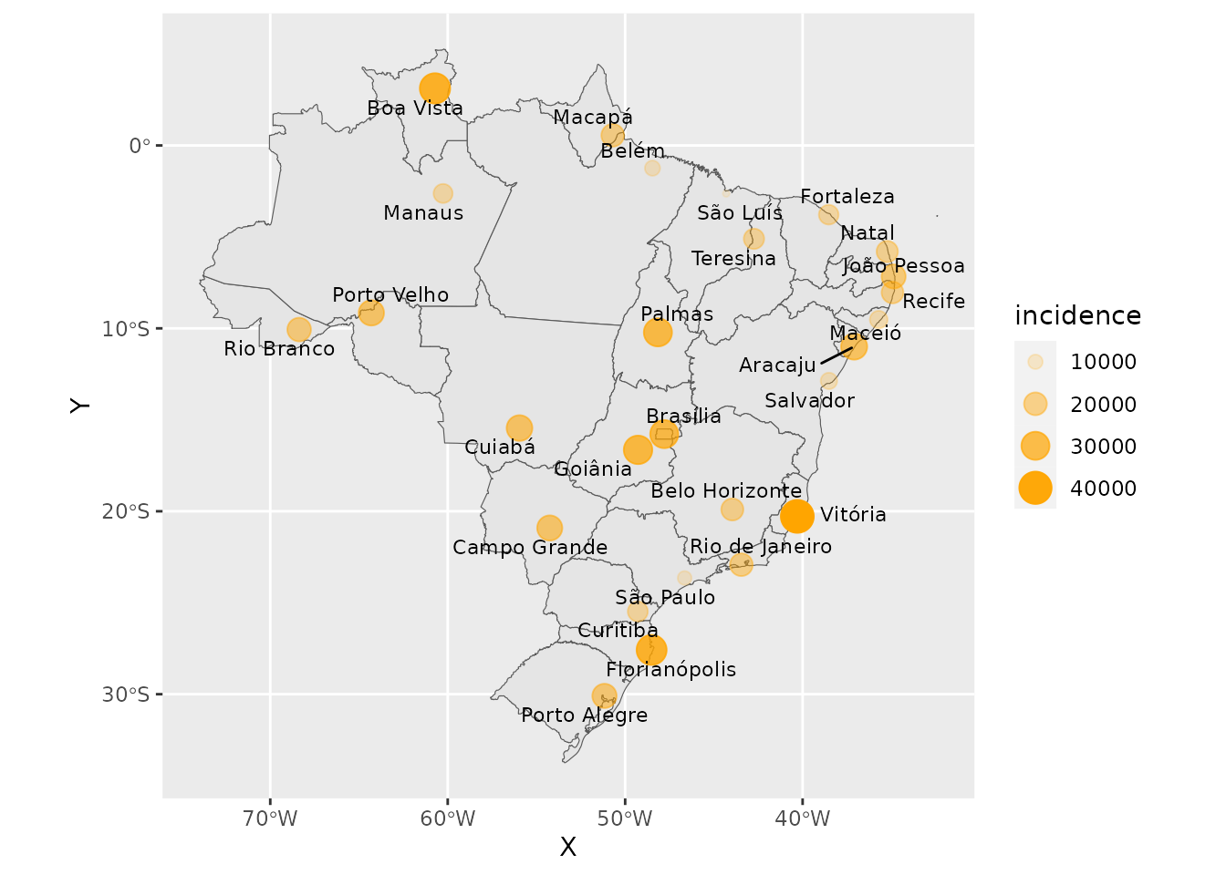
mortality <- ggplot() +
  geom_sf(data = states_geo, aes(geometry=geometry)) +
  geom_point(data = capitals, aes(x=X, y=Y, size=mortality, alpha=mortality), color = "red") +
  geom_text_repel( data=capitals, aes(x=X, y=Y, label=city), size=3)
mortality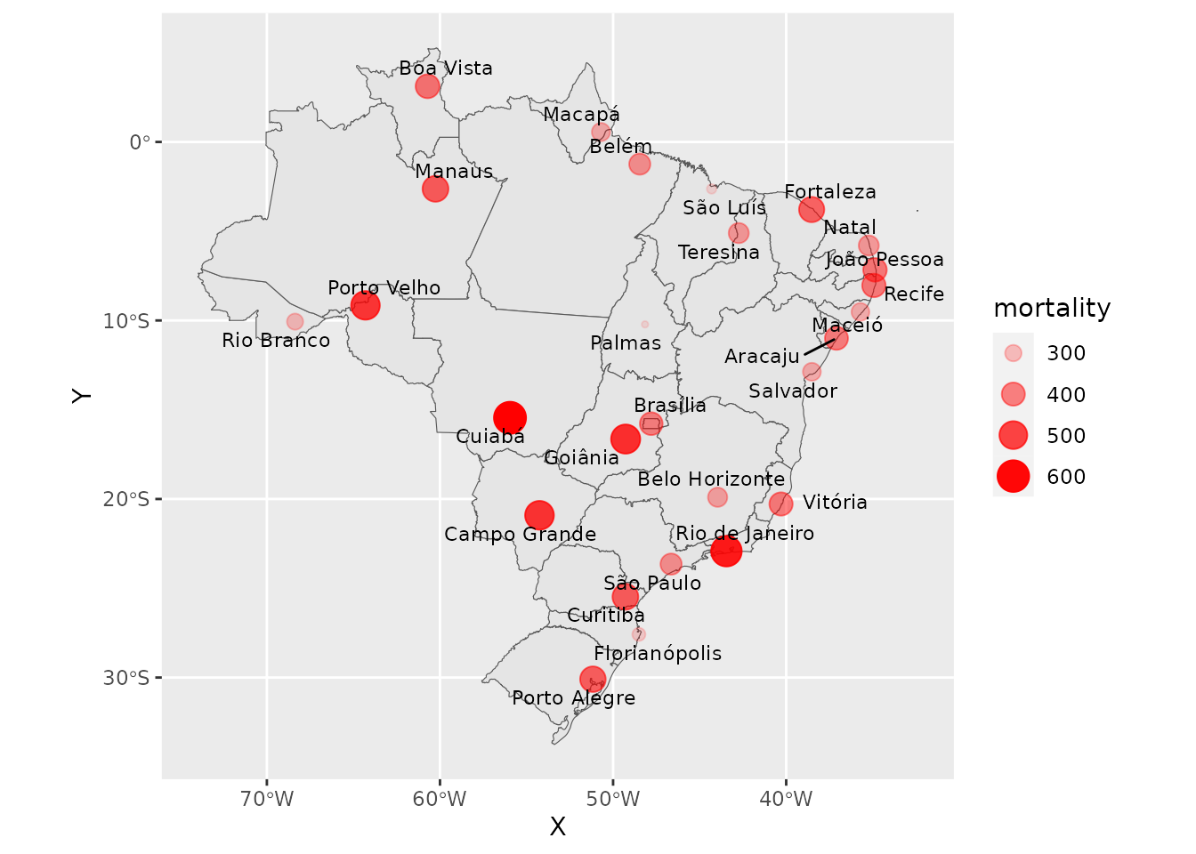
lethality <- ggplot() +
  geom_sf(data = states_geo, aes(geometry=geometry)) +
  geom_point(data = capitals, aes(x=X, y=Y, size=lethality, alpha=lethality), color = "darkred") +
  geom_text_repel( data=capitals, aes(x=X, y=Y, label=city), size=3)
lethality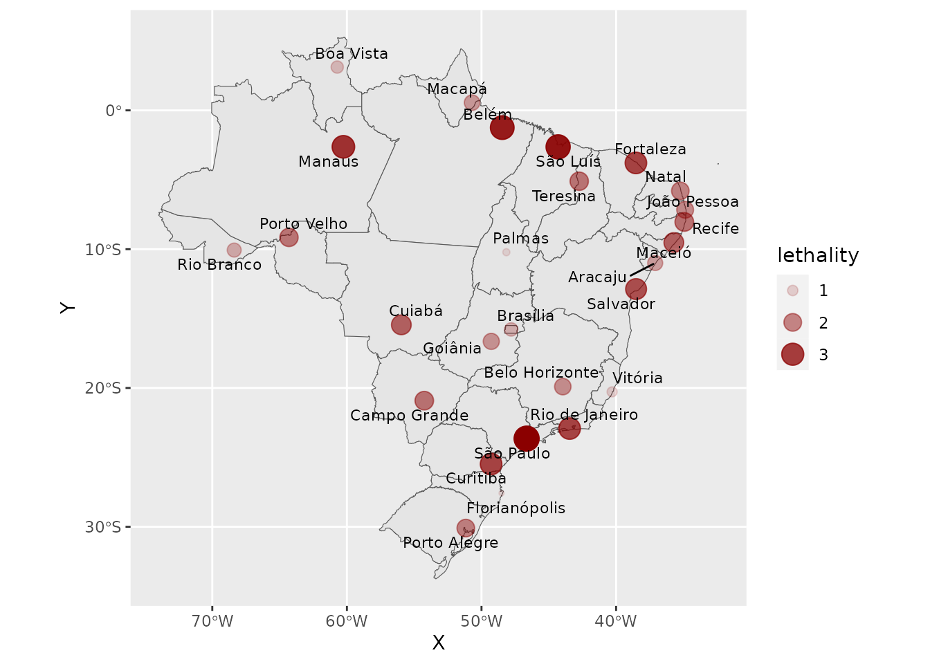
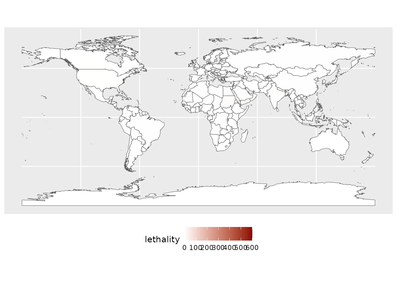
Maps involving world data of COVID-19 pandemic can be draw similarly to the previous examples shown in this vignette. Below we present a simple example:
world <- downloadCovid19("world") %>%
  filter(date == max(date)) %>%
  add_geo() %>%
  add_epi_rates()
#> Downloading COVID-19 data from the Johns Hopkins University's repository
#> Please, be patient...
#> Done!
#> Joining with `by = join_by(country, pop)`

ggplot(world) +
  geom_sf(aes(fill = lethality)) +
  scale_fill_gradient2(low = "red", high = "darkred", na.value = NA) +
  theme(legend.position="bottom")